
Remote sensing has made environmental change increasingly visible.
We can map forest loss, wetland degradation, vegetation stress and land-cover conversion across large areas with growing frequency. Satellites can show where a disturbance occurred, when it began and how its footprint expanded.
But visibility can create a dangerous shortcut.
A mapped hectare of change is often treated as though it represents a consistent environmental consequence. Project reports aggregate the affected area, apply an emission factor and present the result as an estimate of carbon loss or avoided emissions.
The map may be accurate. The conclusion may still be weak.
A change map tells us where something happened. It does not, by itself, tell us how much carbon was affected, whether the loss will persist or whether an intervention restored the value that was lost.
Equal areas can produce unequal consequences
Research reported by the European Space Agency in August 2026 illustrates this gap.
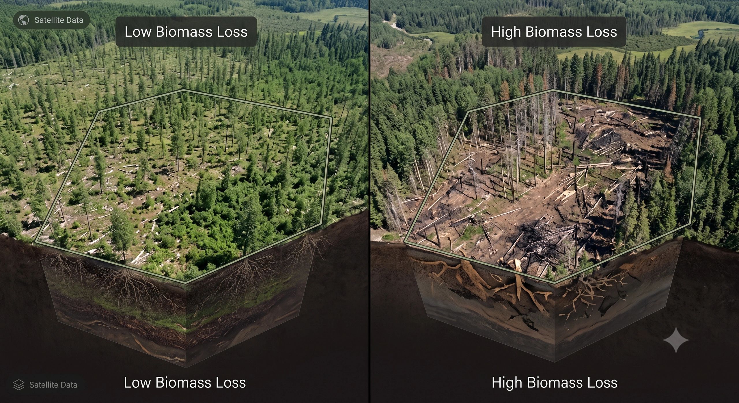
The analysis combined annual tree-cover-loss maps derived from Landsat observations with biomass information. It found that each disturbed hectare in European forests has, on average, been associated with 46% more biomass loss since 2018.
The disturbance footprint alone would not have revealed this change.
Drought, windstorms and insect outbreaks have increasingly affected mature, carbon-rich forests. A disturbance in such a forest can remove substantially more biomass than an event covering the same area in younger or less carbon-dense vegetation.
Consider two forest disturbances, each covering 100 hectares.
The first affects young, regenerating woodland with relatively low biomass density. The second affects mature forest containing decades of accumulated biomass. Their mapped areas are identical, but their carbon implications may differ sharply.
The same principle applies beyond forests.
A hectare of degraded wetland cannot automatically be equated with a hectare of healthy peatland. A plantation cannot be treated as environmentally equivalent to an old-growth ecosystem. Seasonal canopy loss cannot be interpreted in the same way as permanent land conversion.
Area is an essential measurement. It is not the final result.
Detection is only the beginning of MRV
Many environmental monitoring systems are strong at identifying spatial change. They can compare imagery, classify land cover and issue alerts when vegetation is removed or degraded.
The more difficult questions begin after detection:
- What existed at that location before the disturbance?
- How much above-ground and below-ground biomass was present?
- What type and severity of disturbance occurred?
- How much biomass was removed, damaged or left standing?
- Is the loss temporary, recurring or permanent?
- Is natural regeneration likely?
- Could the stored carbon be released gradually rather than immediately?
- Has recovery started, and is it proceeding as expected?
These are not mapping questions alone. They require the integration of Earth observation, ecological baselines, field measurements, accepted carbon methodologies and time-series evidence.
This is why a carbon MRV system cannot stop at change detection. It must convert an observed disturbance into a qualified, traceable and methodologically valid carbon claim.
From change footprint to material consequence
A more decision-ready workflow would connect six evidence layers.
1. Baseline condition
The system must establish what existed before the event: vegetation type, ecosystem maturity, biomass density, carbon pools, land-management history and prior disturbance.
Without a reliable baseline, the meaning of subsequent change remains uncertain.
2. Disturbance footprint
Satellite, aerial or field observations identify where change occurred and establish its timing and spatial extent.
This is the layer that conventional change maps handle well.
3. Disturbance severity
Not every affected pixel represents total loss. Some areas may experience canopy thinning, partial mortality, fire damage or temporary stress. Others may be completely cleared.
Severity determines how much of the baseline biomass was materially affected.
4. Carbon consequence
The observed biomass impact must be translated through an accepted methodology. That process needs to account for relevant carbon pools, uncertainty, leakage, permanence and the timing of possible emissions.
A biomass estimate contributes to the calculation. It should not be presented as a certified carbon result by itself.
5. Recovery trajectory
A one-time post-event image cannot establish whether environmental value has been restored.
Repeated observations should show whether vegetation is regenerating, whether biomass is returning and whether recovery is consistent with the expected trajectory. Field or UAV evidence may be needed where satellite observations remain inconclusive.
6. Intervention history
The system should record what action was taken, who authorized it, when it was completed and what evidence demonstrates its effect.
This connects ecological monitoring with operational accountability.
Together, these layers create a biomass-weighted disturbance record rather than a simple change map.
Why this matters commercially
The distinction affects more than scientific reporting.
For carbon-project developers, weak disturbance accounting can overstate or understate project performance. For buyers, it creates uncertainty about the environmental integrity of the credits being purchased. For insurers and investors, it can hide changes in the real exposure of a forest or restoration portfolio.
Governments also need more than project boundaries and hectare totals. They must understand how land-sector activities affect national carbon budgets, climate commitments and the risk of future reversals.
Supply-chain monitoring faces a similar issue. A company may know that vegetation loss occurred near a sourcing location, but it still needs to determine the ecosystem affected, the severity of the event, its relationship to the supplier and the response required.
The valuable product is therefore not another colored layer on a dashboard.
It is an evidence workflow that connects observation to material impact, obligation, authorized response and verified recovery.
Governance must travel with the measurement
More detailed environmental models do not automatically produce more trustworthy decisions.
Every reported result should retain its provenance:
- imagery and acquisition date;
- biomass dataset and version;
- model or method used;
- assumptions and emission factors;
- confidence and uncertainty;
- field-verification status;
- reviewer and approval history;
- subsequent corrections.
If the baseline changes or a model is updated, the earlier result should not silently disappear. Decision-makers must be able to see what changed, why it changed and whether the revised estimate affects a previously issued claim.
Human review also remains essential. Automated detection can initiate an investigation, prioritize fieldwork and highlight abnormal recovery. It should not silently determine whether a carbon claim is valid, transferable or compliant with a particular programme.
Detection, estimation, verification and authorization are separate functions. A credible MRV architecture should preserve those boundaries.
The next step for environmental intelligence
Remote sensing has solved a major part of the visibility problem. It can repeatedly observe areas that would be expensive or impossible to inspect only from the ground.
The next challenge is to prevent that visibility from being mistaken for a verified outcome.
Decision-grade MRV must explain not only where the landscape changed, but what environmental value was affected, how the conclusion was reached and whether subsequent action restored that value.
A change map is evidence.
A carbon result is a governed conclusion built from multiple forms of evidence.
The future of environmental MRV will depend on how carefully we preserve that distinction.