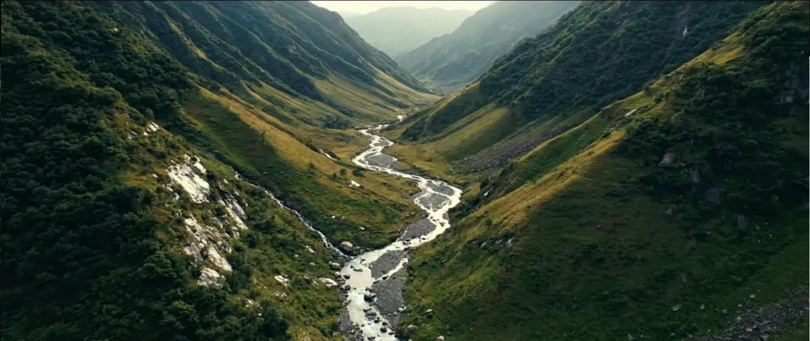
Rivers Don’t Just Flow, They Compute
Every river network is a living algorithm.
The way streams join, split, and merge follows a structured logic, one that mathematicians describe as a graph and hydrologists map as a watershed.
When we translate these networks into nodes and edges, what emerges is not just a map of flow, but a hierarchical data structure that explains how water organizes the landscape.
In essence, watersheds are natural graphs , and Strahler order is their numbering system.
From Drainage Lines to Data Links
A watershed can be modeled as a directed acyclic graph (DAG), where:
Nodes represent confluences or stream junctions.
Edges represent stream segments that carry flow.
Direction indicates the flow from headwater to outlet.
This structure helps hydrologists model everything from stream order to sediment flow and catchment management.
In GIS, this begins with a DEM (Digital Elevation Model) :
Run flow direction and flow accumulation algorithms.
Derive drainage lines and catchment boundaries.
Convert the network into a topological graph , each confluence gets a unique ID and connectivity index.
Once the network is digitized, it can be analyzed like a neural or transportation network, weighted, ranked, and optimized.
The Strahler Stream Order System: Nature’s Hierarchy
Arthur Strahler’s 1952 classification remains the foundation of hydrological graph theory.
Order 1: Headwater streams (no tributaries).
Order 2: Formed when two 1st-order streams merge.
Order 3: When two 2nd-order streams meet, and so on.
If a lower-order stream joins a higher-order stream, the order remains unchanged.
This creates a branching hierarchy that reveals the maturity and complexity of a watershed.
Key insights derived from Strahler order:
Stream Density: Indicates erosional potential and surface runoff.
Bifurcation Ratio (Rb): Ratio of the number of streams of one order to the next, reflects structural control and drainage texture.
Length Ratio (Rl): Reveals energy distribution across the watershed.
Drainage Network Index: A composite measure of hydrological connectivity.
This system turns river geometry into quantifiable data, enabling models that predict flood risk, sediment yield, and channel stability.
From Terrain to Topology: GIS Implementation
Using CartoDEM or SRTM 30m , hydrologists can extract watershed graphs at any scale:
Flow Accumulation Thresholding: Identifies stream initiation points.
Stream Network Vectorization: Converts flow paths into line features.
Topology Building: Detects nodes and connectivity automatically.
Strahler Ordering: Assigned using algorithms (e.g., TauDEM, ArcHydro).
Graph Analytics: Measures centrality, connectivity, and node influence.
With these layers, a watershed becomes not just a hydrological system, but a computable graph , ready for simulation and optimization.
Case Example: Godavari Basin, The Logic of Confluences
The Godavari River , India’s second-longest basin, spans nearly 312,000 sq. km . Using DEM-derived flow accumulation and Strahler ordering, researchers identified:
Order Range: 1 to 8.
Bifurcation Ratio (Rb): 3.2 (moderate structural control).
Drainage Density: 0.95 km/km², showing semi-stable runoff behavior.
By converting this into a hydrological graph , each confluence became a node with weighted attributes, elevation, discharge, and sediment load.
This representation allowed for:
Flood propagation modeling: how peak discharge travels downstream.
Reservoir placement optimization: using network centrality metrics.
Catchment prioritization: identifying critical sub-basins influencing downstream sedimentation.
The result? A data-driven framework for managing a basin not as a single entity, but as a connected network of dynamic nodes.
Graph Thinking in Modern Watershed Management
Viewing watersheds as graphs opens new analytical dimensions:
Connectivity Analysis: Quantify how upstream changes affect downstream nodes.
Resilience Modeling: Identify nodes most critical to flood resilience.
Sediment Pathways: Simulate how material moves through channel hierarchies.
Water Quality Flow: Model pollutant propagation through a directed network.
In essence, hydrology meets data science, and the watershed becomes a living computational system.
GeoAI and Stream Network Intelligence
AI models now interpret these natural graphs automatically:
CNNs on DEM data: Extract stream networks without manual delineation.
Graph Neural Networks (GNNs): Learn relationships between nodes, predicting flow characteristics or erosion risk.
Digital Twin Integration: Hydrological twins simulate water flow dynamically, updating as rainfall or land use changes.
Such systems evolve from simple flow routing models into adaptive hydrological networks , capable of self-learning and real-time prediction.
Outlook: Watersheds as Living Networks
The future of water management will treat every basin as a spatial knowledge graph , linking terrain, hydrology, and socio-economic factors.
Imagine a “Watershed Twin” where each confluence node carries not only flow data, but also population, infrastructure, and land use, allowing planners to assess who is affected downstream in real time.
That’s the next leap, from hydrological graphs to governance graphs.
Conclusion
Watersheds are more than drainage systems, they’re nature’s way of encoding connectivity.
By mapping streams as graphs and decoding their hierarchies through Strahler order, we reveal how water organizes, communicates, and balances energy across the landscape.
In data terms, every river network is a conversation, and the confluence is where nature decides what flows next.