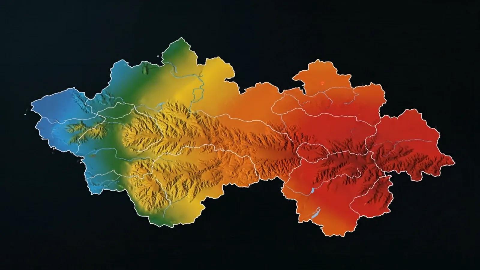
From terrain hints to actionable risk surfaces
Landslides don’t arrive unannounced; the landscape telegraphs them. Gradients steepen, soils thin, drainage concentrates, and rock fabric weakens. Landslide Susceptibility Modeling (LSM) converts these cues into a map of where failure is likely, so planners, road engineers, utilities, and disaster teams can act before slopes do.
What we model (and why it matters)
A robust LSM integrates conditioning factors (long-term predisposition) and triggers (short-term forces):
Core conditioning factors (from DEM, geology, land cover, proximity layers):
Topography: slope, aspect, plan/profile curvature, TPI/TRI (position/roughness), TWI (wetness), relative relief.
Material: lithology, soil type, weathering grade, geomorphology, regolith thickness (if available).
Hydrology: drainage density, distance to streams, convergent flow zones, perched water indicators.
Structure: distance to faults/lineaments, fracture density, bedding–slope relation (dip-slope risk).
Land use / cover: vegetation (NDVI), deforestation, quarrying, agriculture terraces, built-up.
Proximity to intervention: distance to roads/cut-slopes, buildings, pipelines.
Triggers (temporal):
Rainfall intensity/duration (ID thresholds), cumulative antecedent rainfall , soil moisture (satellite or in-situ), earthquakes (PGA/PGV).
Three modeling families (pick for context, data, and scale)
Heuristic / knowledge-driven
Weighted Overlay, AHP (Analytic Hierarchy Process): experts assign weights/scores to factors/classes.
Pros: transparent, quick with sparse data; easy to communicate.
Cons: subjective; difficult to capture nonlinear interactions.
Statistical / classical ML
Logistic Regression, WOE/FR (Weights of Evidence / Frequency Ratio): quantify correlation of factors with mapped landslides.
Tree ensembles (RF, XGBoost, LightGBM): capture nonlinearities and interactions; strong baselines.
Pros: good accuracy, interpretable (LR, WOE) or explainable (SHAP for trees).
Cons: risk of overfitting; needs careful validation and balanced training data.
Deep learning / spatial DL
CNN/UNet on rasters; GNNs on slope units: learn spatial patterns from imagery + DEM derivatives.
Pros: highest representational power at large scales.
Cons: data-hungry, heavier MLOps, explainability needed for policy use.
Mapping unit, resolution, and sampling
Pixel-based (e.g., 10–30 m): best for wall-to-wall coverage; risk of spatial autocorrelation bias.
Slope-unit / catchment-unit : aggregates pixels into process-consistent polygons, often improves generalization.
Match resolution to process scale and inventory accuracy (don’t upsample truth).
Handle class imbalance (few landslide pixels vs many stable) via stratified sampling , SMOTE , or class weights .
Building the inventory (the model lives or dies here)
Compile multi-temporal landslide polygons/points from field mapping, high-res imagery, or UAVs.
Distinguish training period (older events) and validation period (recent events) to avoid temporal leakage.
Separate by event type where possible (debris flow, rockfall, deep-seated), or model a unified “susceptible/not” with type as an attribute.
Feature engineering & sanity checks
Derive slope, aspect, curvature, TPI/TRI, TWI from DEM; compute distances (faults, roads, streams); stack NDVI/land-use.
Remove multicollinearity (e.g., slope vs relief) using VIF/Correlation pruning.
Encode categorical geology with one-hot or target encoding.
Normalize/standardize where the model requires it.
Model training and validation that actually holds up
Don’t trust random k-fold alone; spatial data leaks. Use spatial and temporal validation :
Spatial k-fold / block CV: hold out spatial blocks or entire sub-basins/tehsils to test transferability.
Temporal split: train on pre-T date; validate on post-T events (e.g., after a monsoon season).
Metrics: ROC-AUC for ranking ability; PR-AUC when positives are rare. TSS (sensitivity + specificity − 1) for thresholded maps. Brier score / reliability diagrams for probability calibration.
Calibration: isotonic regression or Platt scaling so “0.7” actually means 70% likelihood.
Uncertainty: produce prediction intervals (quantile forests) or ensemble spread (RF/XGB/UNet committee).
Explainability: SHAP values (or LR coefficients) to show drivers (e.g., slope, TWI, distance-to-road).
Turning scores into a map people can use
Classify susceptibility (Very Low → Very High) with quantiles or Jenks natural breaks ; publish both the continuous probability and the classed map .
Overlay exposure (settlements, roads, lifelines) to derive risk = susceptibility × exposure .
Generate action layers : Priority micro-zonation for road cut stabilization. No-build/conditional-build buffers. Drainage/retaining measures and afforestation zones.
Package outputs in GeoPackage/3D Tiles and a simple web map for ops teams.
Indian context (Himalaya + NE + Western Ghats)
Himalaya/Siwalik: high slopes, active thrusts (MBT/MCT), strong monsoon intensities → debris flows and rockslides.
NE India: high rainfall, deeply weathered lithologies; drainage density a strong driver.
Western Ghats: lateritic caps + road cuts; NDVI loss + curvature + distance-to-road often top features.
Use CartoDEM/SRTM/ALOS , Sentinel-1 (soil moisture proxy; wetness) , IMD rainfall , GSI geology , NRSC land use for national-scale stacks.
Common pitfalls (and quick fixes)
Pixel leakage: Use spatial/temporal CV; prefer slope-unit modeling.
Imbalanced truth: Tune thresholds for recall in High/Very-High classes; communicate trade-offs.
Over-interpretation: Susceptibility ≠ hazard timing; pair with rainfall triggers for nowcasting .
Black-box resistance: Publish SHAP charts + factor response curves; keep a lightweight AHP/FR baseline for auditability.
Road to deployment and early warning
Nightly ETL : ingest rainfall (IMERG/IMD), soil moisture (Sentinel-1), and update nowcast layers on top of the base susceptibility.
Alerts where (High class) AND (24–72 h rainfall > threshold) .
Track outcomes (hit/miss) → continual learning loop.
Conclusion
An LSM is not just a pretty heatmap. It’s a decision instrument that converts terrain physics and human footprints into prioritized actions, where to stabilize, where not to build, and when to warn. With sound inventories, factor discipline, and spatial-temporal validation, susceptibility maps become credible foundations for resilient planning.