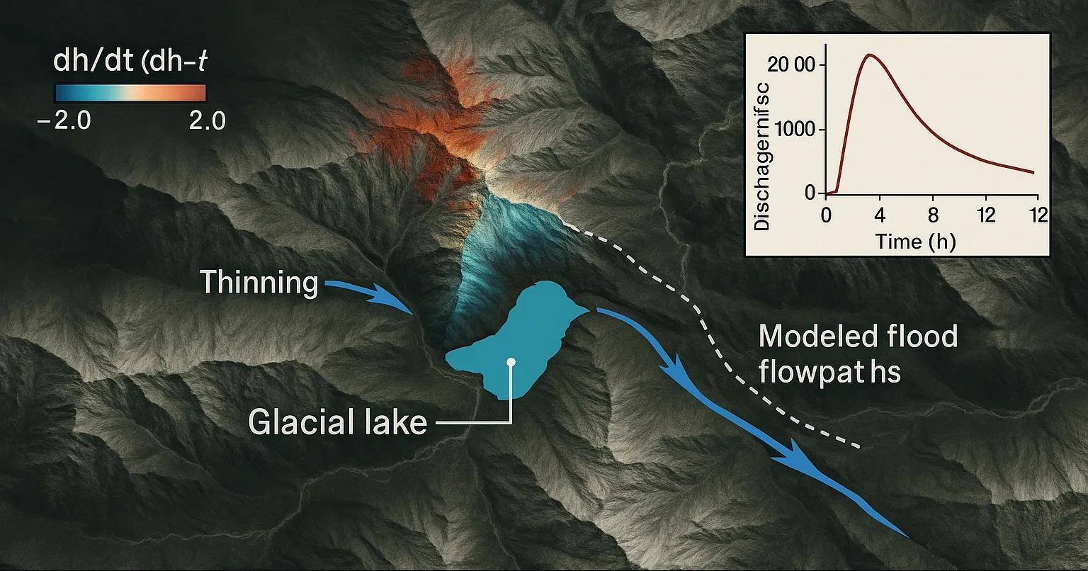
When Meltwater Becomes a Mountain Hazard
As Himalayan glaciers thin and retreat, meltwater pools behind loose, unconsolidated moraine walls. These glacial lakes are not lakes in the traditional sense, they are temporary, unstable reservoirs formed by climate change.
When a moraine dam fails, the sudden release of water forms a Glacial Lake Outburst Flood (GLOF) , a fast-moving wall of debris-laden water capable of destroying bridges, hydropower assets, and entire villages downstream.
Understanding GLOF risk requires quantifying three things :
How much water the lake stores (volume)
How likely the moraine is to breach
How far and how fast the flood will travel
Geospatial analytics now provides answers to all three.
Mapping Glacial Lakes: The First Layer of Risk Intelligence
Using multispectral and SAR imagery, glacial lakes can be precisely delineated:
Sentinel-2 (10 m): Ideal for surface mapping through NIR/SWIR indices
PlanetScope (3–5 m): High-resolution for small or newly formed lakes
Sentinel-1 SAR: Detects lake area even under cloud cover
ASTER & Landsat archives: Enable time-series growth assessment since the 1990s
Most lakes in the Eastern Himalaya (Sikkim, Arunachal) show rapid expansion , while those in Himachal and Uttarakhand are forming more slowly but are structurally more sensitive due to steep valley gradients.
Estimating Lake Volume: The Key Step in GLOF Modeling
Surface area alone cannot indicate risk, what matters is volume , the potential flood load.
Three common geospatial approaches are used:
1️⃣ Empirical Area–Volume Equations
Derived using global datasets of known glacial lakes:
V = a⋅A^b
Where A = area and a, b are coefficients calibrated for Himalaya-specific morphology.
2️⃣ Bathymetry from DEM Differencing
For lakes whose bottoms were exposed in previous DEMs (e.g., SRTM 2000):
Subtract past terrain DEM from current water-surface DEM
Gives approximate basin depth → volume
3️⃣ UAV/LiDAR Surveys (High Confidence)
Drones with bathymetric LiDAR or photogrammetry give 0.1–0.3 m accuracy.
Used in high-risk lakes like South Lhonak (Sikkim) and Tsho Rolpa (Nepal) .
Volume estimates feed directly into downstream flood simulations.
Moraine Stability: The Weakest Link
A glacial lake dam is usually a pile of poorly sorted rock, sand, and ice. Breach susceptibility depends on:
Dam composition (ice core? boulder-rich? loosely packed?)
Freeboard (height difference between lake surface and dam crest)
Seepage channels
Slope and oversteepened downstream face
Avalanche or rockfall exposure
Geospatial inputs used:
Sentinel-1 SAR coherence → detects dam instability
Slope & aspect from DEM → hazard geometry
Thermal anomalies → reveals ice-cored moraines
Proximity to steep hanging glaciers → avalanche potential
These parameters are combined into a Moraine Breach Susceptibility Index (MBSI) .
Breach Hydrographs: How GLOF Models Are Built
Once volume and dam stability are known, breach scenarios can be simulated through hydrodynamic models like:
HEC-RAS 2D
DHI MIKE-11 / MIKE-21
BASEMENT
Inputs include:
Lake volume
Dam breach width + depth
Breach formation time (minutes to hours)
Downstream valley DEM
Manning’s roughness coefficients
Outputs include:
Peak discharge ( Qpeak )
Arrival time at downstream assets
Flood depth maps
Impact zones on roads, bridges, hydropower stations
These maps are vital for early warning systems across Himalayan states.
Case Example: South Lhonak Lake, Sikkim (2023 GLOF Event)
Pre-2023 satellite analysis showed:
Rapid expansion: 65% growth between 2010–2023
Multiple trigger zones: avalanche-prone slopes & supra-glacial debris
Low freeboard and weakened moraine
A sudden avalanche on the night of 3 October 2023 caused a dam breach, sending a massive flood downstream through Teesta River.
Post-event analysis using Sentinel-1 SAR & HEC-RAS indicated:
Estimated lake volume: ~55 million m³
Peak discharge: 10,000–20,000 m³/s
Dam eroded rapidly within minutes
This emphasized the need for dynamic monitoring , not static inventories.
GeoAI for GLOF Forecasting
Machine learning models are now improving glacial lake hazard assessment by:
Automatically detecting lake expansion (NDWI, MNDWI + CNN classifiers)
Predicting breach probability using historical GLOF datasets
Mapping unstable moraine zones through SAR temporal coherence
Generating synthetic breach scenarios using data-driven surrogates
Future applications include near-real-time lake monitoring fed by:
PlanetScope daily imagery
Sentinel-1 6-day SAR
ICESat-2 elevation updates
UAV periodic surveys
Toward Glacial Lake Digital Twins
A Glacial Lake Digital Twin integrates:
Lake area and volume time-series
DEM evolution
Ice-melt and avalanche triggers
Moraine stability indicators
Hydrodynamic flood simulation models
This enables:
Continuous hazard scoring
Early warnings
Scenario-based emergency planning
Infrastructure risk analytics (bridges, hydropower, roads)
India’s Himalayan states are beginning to integrate such systems into disaster management dashboards .
Conclusion
Every glacial lake is both a water reserve and a potential hazard.
With SAR, ICESat-2, DEM differencing, and hydrodynamic models, we can now quantify both, the stored volume and the catastrophic potential.
GLOF risk is no longer unpredictable, it is a spatial problem with measurable signals.