Mapping Life Like Data
Every species leaves a trace, a presence record, a range map, a pixel of life.
When thousands of these traces are assembled across landscapes, they form spatial layers of biodiversity , digital habitats that can be modeled, mapped, and monitored.
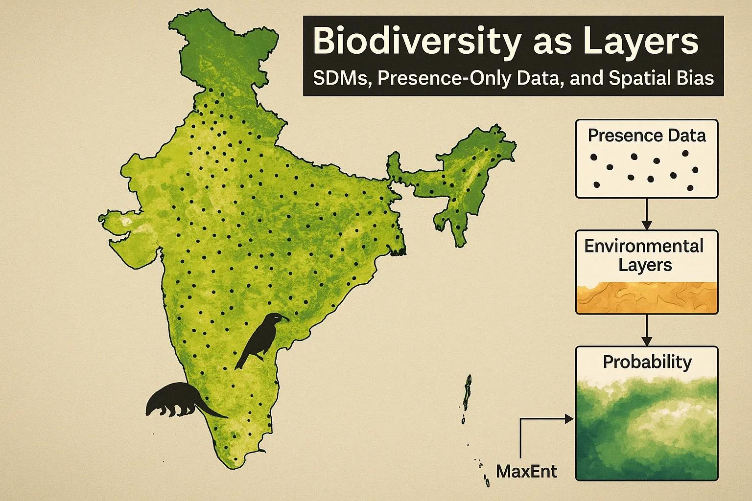
This is the domain of Species Distribution Models (SDMs) , geospatial tools that use occurrence data and environmental variables to estimate where species can and do exist.
In essence, SDMs convert biology into probability, turning field sightings into maps of ecological potential.
The Core Idea: Predicting Habitat Suitability
An SDM links species presence data (from observations or museum records) with environmental layers such as:
Elevation (DEM)
Land cover and NDVI
Temperature and precipitation (BIOCLIM variables)
Soil type and topography
From these inputs, models learn the environmental envelope a species occupies, and project it across space.
P ("occurrence") = f ("environmental variables")
This probability surface becomes a habitat suitability map , predicting where conditions are favorable even if direct observations are absent.
The Challenge: Presence-Only Reality
In an ideal world, we’d have both presence and absence data, knowing not only where a species is found, but also where it’s confirmed to be absent.
In reality, most biodiversity data are presence-only , citizen sightings, herbarium records, GBIF entries, all documenting where something was seen, not where it wasn’t.
This limitation shaped the rise of algorithms like MaxEnt (Maximum Entropy) , the workhorse of presence-only SDMs.
MaxEnt Principle: Predicts species distribution by finding the probability distribution of maximum entropy (least bias) constrained by known environmental conditions at presence points.
Why it works: It assumes that, given limited knowledge, the best prediction is the least biased one, consistent with what we know, but not assuming more.
Handling Bias: When Data Cluster Around Roads
Presence-only data are rarely random.
Observation density often follows human accessibility , roads, cities, research zones, leading to sampling bias .
For example:
Birds reported more often near birding hotspots than remote forests.
Mammal data biased toward protected areas.
Marine species sightings clustered near coasts or shipping lanes.
This bias inflates model accuracy where sampling is dense, while underestimating suitability in underexplored regions.
Mitigation Techniques:
1️⃣ Spatial Filtering: Remove duplicate or clustered records within a given radius (e.g., 5 km).
2️⃣ Bias Grids: Weight background points by sampling intensity (e.g., from eBird effort maps).
3️⃣ Target-Group Background: Use background data from taxa surveyed under similar effort conditions.
4️⃣ Cross-validation by geography: Partition data by regions, not random subsets.
Correcting bias isn’t optional, it defines whether your map shows species ecology or observer geography .
India’s Biodiversity Data Landscape
India’s biodiversity data is both rich and uneven.
GBIF: >6 million occurrence records.
ZSI & BSI: Extensive museum collections but uneven digitization.
Citizen Science Platforms: eBird, iNaturalist, India Biodiversity Portal, huge data volume but variable spatial coverage.
Remote Sensing Layers: MODIS NDVI, WorldClim, SoilGrids, Copernicus LULC, provide consistent environmental covariates.
Integrating these into SDMs allows researchers to predict species richness , endemism , and climate vulnerability hotspots, key for conservation zoning and protected area design.
Case Example: Modeling the Range of the Indian Pangolin
A 2022 study combined 97 presence records of Manis crassicaudata (Indian Pangolin) from GBIF and WII datasets with 19 bioclimatic variables.
Using MaxEnt with spatial bias correction, researchers found:
Habitat suitability linked strongly to precipitation seasonality and forest cover.
High probability zones in Western Ghats, central India, and Odisha forests.
Range contraction under future RCP 8.5 scenario by up to 40%.
This model guided conservation priorities and anti-poaching patrol planning under the Integrated Biodiversity Conservation Network (IBCN) .
From SDMs to Stacked Biodiversity Layers
When multiple SDMs are combined, they create biodiversity richness maps , summing habitat probabilities across species.
These “stacks” reveal areas of high ecological overlap , often aligning with ecoregions, corridors, or unprotected biodiversity hotspots.
Applications include:
Protected Area Expansion: Identify gaps in conservation coverage.
Climate Adaptation: Forecast species range shifts.
Ecosystem Services: Map pollinator or carbon-storage co-benefits.
When linked to Digital Twins of landscapes , these models could enable dynamic biodiversity monitoring , not just mapping species, but tracking their shifts in near real time.
GeoAI and Next-Gen Biodiversity Modeling
AI is advancing SDMs from statistical projections to learning-based habitat intelligence :
CNNs (Convolutional Neural Networks): Learn spatial patterns directly from remote-sensing imagery.
Graph Neural Networks: Model ecological connectivity between habitat patches.
Spatio-temporal SDMs: Predict distribution changes through time-series environmental data.
Explainable AI (XAI): Helps interpret which variables truly drive species presence.
These tools bridge ecology and informatics , turning biodiversity into a quantifiable and predictive layer in geospatial systems.
Outlook: Toward a Biodiversity Digital Twin for India
Imagine a Biodiversity Digital Twin integrating:
Species occurrence (GBIF, iNaturalist).
Environmental layers (WorldClim, MODIS).
Land use change forecasts.
Genetic and ecological network data.
Such a twin could simulate:
Species shifts under climate and land-use scenarios.
Conservation corridor stability.
Real-time ecosystem health metrics.
India’s National Mission on Biodiversity and Human Well-Being (NMBHWB) could anchor this twin, connecting research, citizen science, and policy.
Conclusion
Every point of species presence is a pixel of life, together, they form the mosaic of our planet’s biological intelligence.
Species Distribution Models are not just about mapping animals or plants, they’re about visualizing how life interacts with space, climate, and change.
When we treat biodiversity as a spatial layer, we begin to manage ecosystems with the same precision we apply to infrastructure or climate, with data as the common language.